Meta AI just introduced Brain2Qwerty v2. It decodes natural sentences from non-invasive brain recordings in real time. The system reads magnetoencephalography (MEG) signals while a person types. It reconstructs what they typed, with no implant and no surgery. This is the follow-up to Brain2Qwerty v1, released in February 2025. Meta is also releasing the full training code for both versions. The pipeline combines a convolutional encoder, a transformer, and a character-level language model.
TL;DR
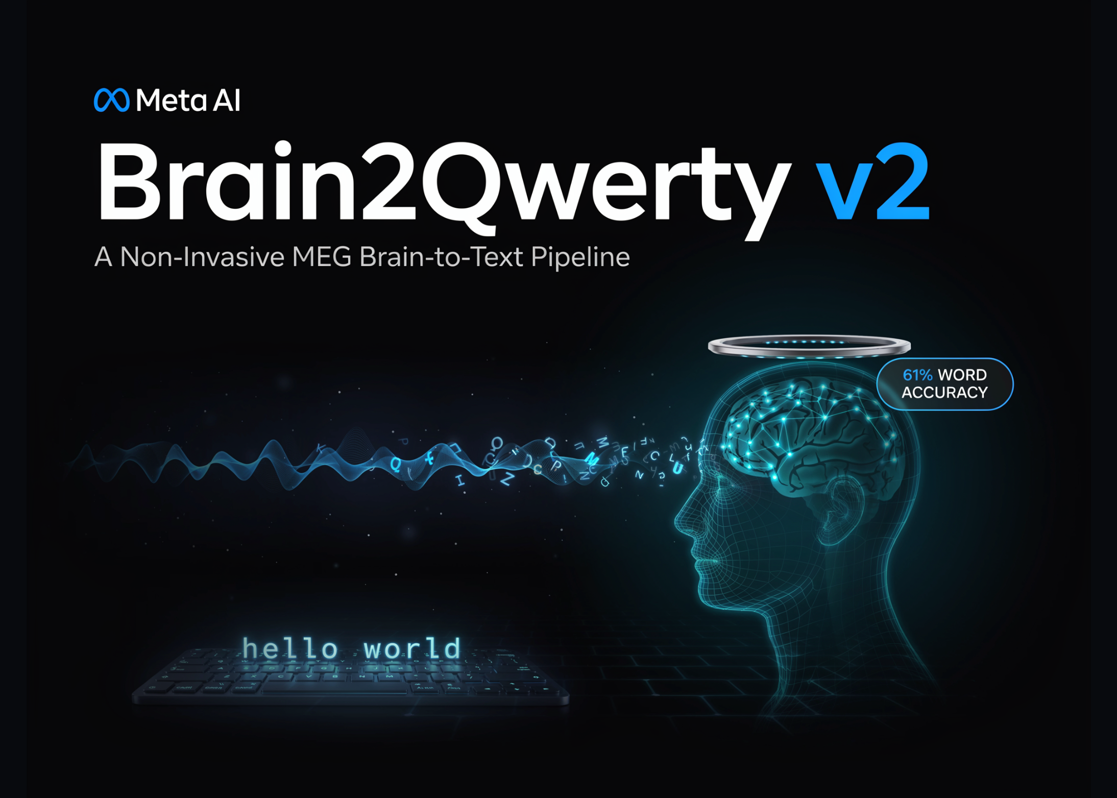
- Brain2Qwerty v2 decodes typed sentences from non-invasive MEG signals, with no implant or surgery.
- It reaches 61% average word accuracy (39% WER), up from 8% for prior non-invasive methods.
- The best participant hit 78% word accuracy, with over half of sentences at one word error or less.
- The pipeline pairs a convolutional encoder, transformer, and character-level language model, plus fine-tuned LLMs.
- Accuracy scales log-linearly with data; training code for v1 and v2 is released under CC BY-NC 4.0.
What is Brain2Qwerty v2?
Brain2Qwerty v2 is a brain-to-text decoder. It maps raw brain activity to characters, then to words and sentences.
Meta trained it on approximately 22,000 sentences from nine volunteer participants. Each participant was recorded for 10 hours while actively typing.
Recordings come from a MEG device. MEG measures the magnetic fields produced by neuronal activity, sampled at high temporal resolution.
The model leverages character, word and sentence-level representations. That layered design lets it correct local errors using broader context.
Importantly, this is research, not a product. The decoder is not a consumer device, and it was tested on a small group of volunteers.
The data was collected with Spain’s BCBL (Basque Center on Cognition, Brain and Language). It belongs to that research center.
How the Decoding Pipeline Works
Earlier non-invasive systems relied on hand-crafted pipelines to detect neural events. Brain2Qwerty v2 replaces that step with end-to-end deep learning.
Per Meta’s repository, the model combines three components: a convolutional encoder, a transformer, and a character-level language model.
The convolutional encoder reads raw MEG signals. It learns features directly from the data instead of using engineered event detectors.
The transformer models longer-range structure across the signal. The character-level language model then constrains the output toward plausible text.
Meta research team describes three ways AI enables the result. Each maps to a concrete engineering decision teams will recognize.
- Deep learning replaces hand-crafted event detection.
- Large language models are fine-tuned to extract semantic representations.
- AI agents iteratively refined the decoding pipeline through automated code development. Final training configurations were still selected manually by devs
Fine-tuning large language models on neural data adds semantic context. That context bridges noisy brain recordings and coherent language output.
In practice, the language model rejects character sequences that form no real words. It pushes the decoder toward sentences a human would plausibly type.
Here is an illustrative sketch of the published architecture. It mirrors the described components and is not Meta’s exact training code.
import torch
import torch.nn as nn

class Brain2QwertySketch(nn.Module):
    """Illustrative: convolutional encoder -> transformer -> char-level head.
    Reflects the components Meta describes, not the official implementation."""
    def __init__(self, n_meg_channels=306, d_model=256, n_chars=40):
        super().__init__()
        # 1) Convolutional encoder over raw MEG channels x time
        self.encoder = nn.Sequential(
            nn.Conv1d(n_meg_channels, d_model, kernel_size=7, padding=3),
            nn.GELU(),
            nn.Conv1d(d_model, d_model, kernel_size=5, padding=2),
            nn.GELU(),
        )
        # 2) Transformer models temporal structure
        layer = nn.TransformerEncoderLayer(d_model, nhead=8, batch_first=True)
        self.transformer = nn.TransformerEncoder(layer, num_layers=6)
        # 3) Character-level head; a language model refines this downstream
        self.char_head = nn.Linear(d_model, n_chars)

    def forward(self, meg):           # meg: (batch, channels, time)
        x = self.encoder(meg)         # (batch, d_model, time)
        x = x.transpose(1, 2)         # (batch, time, d_model)
        x = self.transformer(x)       # contextualized features
        return self.char_head(x)      # (batch, time, n_chars)
To work with Meta’s real code, clone the repository and inspect both versions:
git clone https://github.com/facebookresearch/brain2qwerty
# brain2qwerty_v1/ and brain2qwerty_v2/ hold the training code
The Accuracy Numbers
Brain2Qwerty v2 achieves an average word accuracy rate of 61%. That corresponds to a word error rate (WER) of 39%.
For the best participant, the model reaches 78% word accuracy. For that participant, over half of sentences had one word error or less.
The prior baseline matters here. Meta reports that other non-invasive methods reached only 8% word accuracy.
Accuracy also improves log-linearly with data volume. More recording hours predictably raise accuracy in the reported range.
That scaling behavior is the key claim for builders. It suggests the gap with surgical implants could narrow through data alone.
| Metric | Brain2Qwerty v2 | Prior non-invasive methods |
|---|---|---|
| Average word accuracy | 61% | 8% |
| Average word error rate (WER) | 39% | — |
| Best participant word accuracy | 78% | — |
| Recording method | MEG, non-invasive | Non-invasive |
| Scaling behavior | Log-linear with data | — |
These numbers come from volunteers in a controlled setting. They are not clinical results for patients with brain injuries.
v1 vs v2: What Changed
Brain2Qwerty v1 and v2 report different metrics, so compare them carefully. v1 was measured at character level, v2 at word level.
| Aspect | Brain2Qwerty v1 (Feb 2025) | Brain2Qwerty v2 (Jun 2026) |
|---|---|---|
| Devices | MEG and EEG | MEG |
| Participants | 35 healthy volunteers | 9 volunteers |
| Data | Typed sentences | ~22,000 sentences, 10 hours each |
| Reported result | Up to 80% of characters (MEG) | 61% average word accuracy |
| Representation level | Character-level | Character, word and sentence-level |
| Real-time decoding | Not emphasized | Real-time sentence decoding |
v1 also showed MEG decoding was at least twice better than the EEG system. EEG signals are noisier, which limits accuracy.
Use Cases With Examples
- The primary motivation is restoring communication. Millions of people have brain lesions that prevent them from speaking or moving.
- Invasive methods like stereotactic electroencephalography and electrocorticography already feed a neuroprosthesis to an AI decoder. But they require neurosurgery and are hard to scale.
- A non-invasive decoder could widen access. A patient could potentially type sentences without an implant, using only external recordings.
- For researchers, the released code supports reproducible neuroscience. A lab could retrain the pipeline on its own MEG dataset.
- For AI engineers, the project is a template for biosignal decoding. The convolutional-encoder-plus-transformer pattern transfers to other biosignal tasks.
- For data scientists, the log-linear scaling result is a planning tool. It frames how much new recording data may lift accuracy.
Interactive Explainer